Groth-Sahai Proofs Are Not That Scary

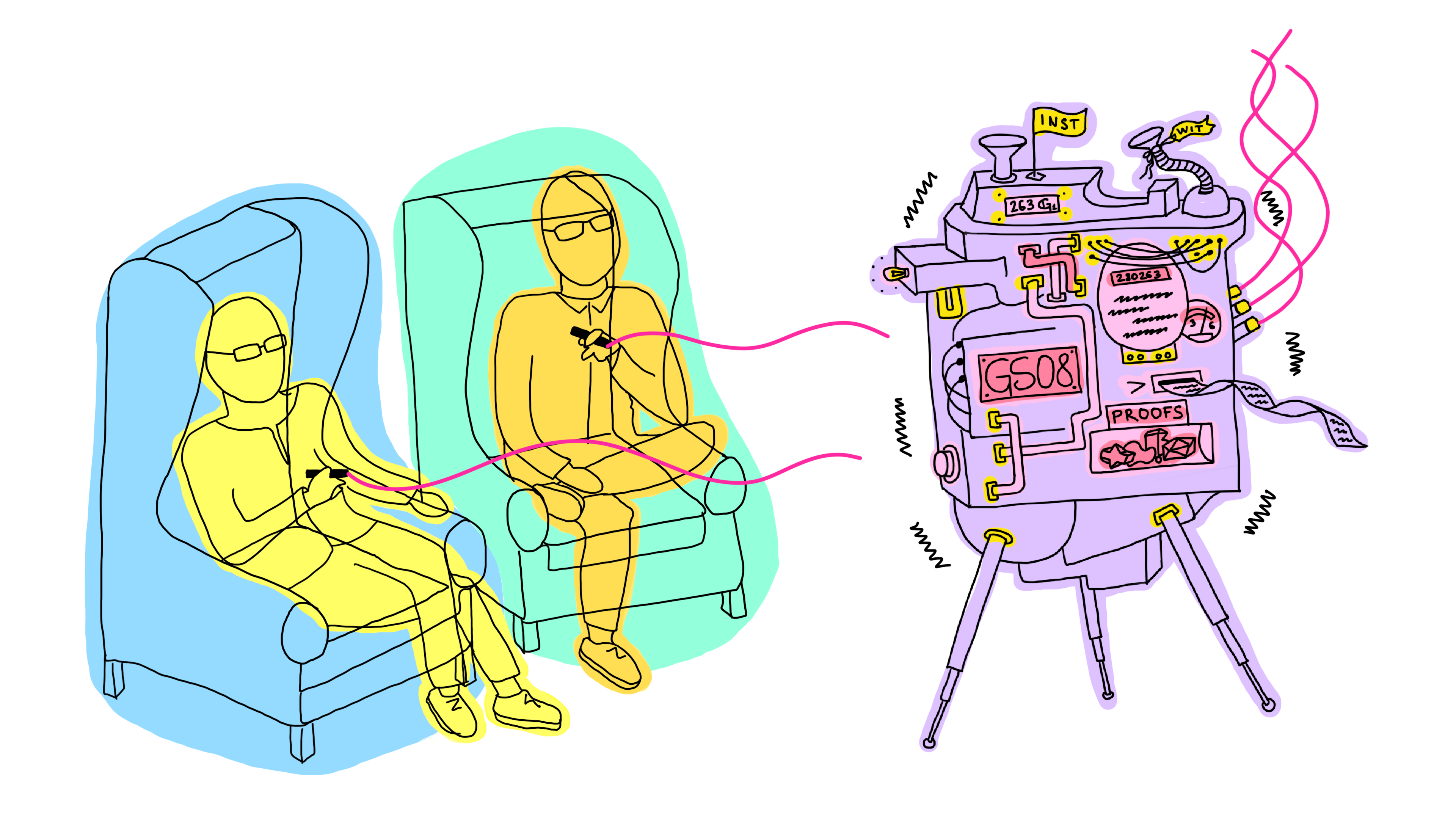
Mikhail Volkhov, Dimitris Kolonelos, Dmitry Khovratovich, Mary Maller | June 6, 2022

Groth-Sahai (GS) proofs are a zero-knowledge proving technique which can seem daunting to understand. This is because much of the literature attempts to generalise all possible things you can prove using GS techniques rather than because the proofs are overly complicated. In fact GS proofs are one of the simplest zero-knowledge constructions. For statements about group elements in pairing based groups, they are ideal because there is no heavy reduction to an NP constraint system, and this makes the prover very fast. Security wise they also rely on much more standard assumptions than SNARKs and thus are more likely to be secure.

In this post we will walk through an example Groth-Sahai proof and attempt to make the explanation accessible to a general cryptographic audience. Specifically we discuss how to prove that an ElGamal ciphertext contains $0$ or $1$. Our example includes the improvements by Escala and Groth. Prerequisites include knowledge about what a zero-knowledge argument is and what Type-III pairings are (but not how they are constructed).

And for those interested in experimenting with GS proofs in practice we have written a simple implementation in python -- check it out! It includes both the example we will be going through in this paper, and the more general proving framework that you can use to construct proofs for your language.

ElGamal in Pairing Product Equations

In order to prove that an ElGamal ciphertext contains $0$ or $1$ we must first arithmetise this statement into a form that is compatible with GS proofs. GS proofs take as input pairing-product equations; pairing product equations can be seen as the equivalent of arithmetic circuits in the sense that they arithmetise the relation that we are trying to prove. Thus in this section we show how to represent our statement using pairing product equations. In later sections we will show how to prove that these equations are satisfied under zero-knowledge.

Notation and Pairings

Recall the standard property of pairings: $e(g^a,\widehat{h}^b) = e(g,\widehat{h})^{ab}$ We denote the first source group by $\mathbb{G}_1$ and the second source group by $\mathbb{G}_2$. Elements from $\mathbb{G}_2$ are denoted with wide hat like $\widehat{E}$. We will write $\Theta = g^{\theta}$ and $\widehat{D} = \widehat{h}^d$ trying, where it's possible, to use lowercase letters for exponents of the corresponding capital letter element.

Pairings allow us to define quadratic equations in the logarithms of the arguments, e.g.

If you have not worked with pairings with multiple bases, see this explanation:

Collapsible: On Pairings with Multible Bases

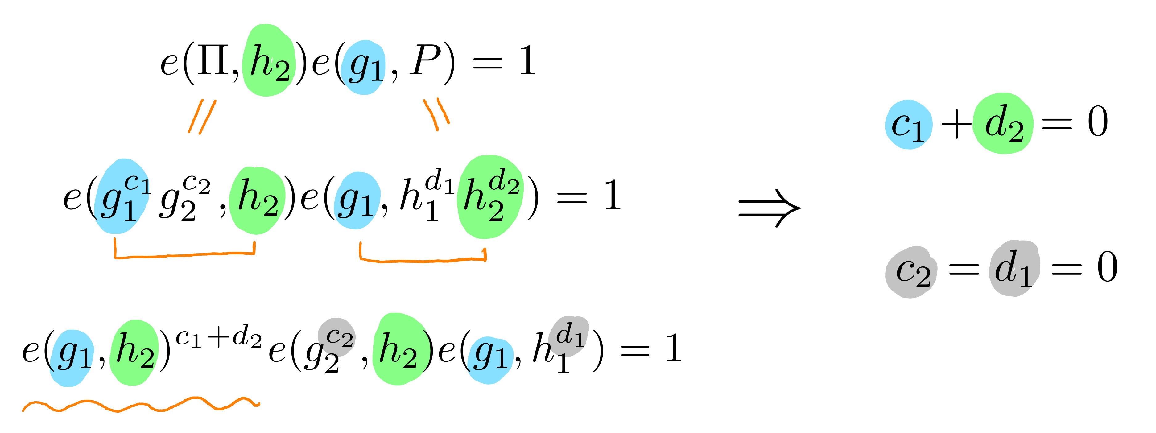
As later we will employ multiple bases and not just $g,\widehat{h}$, pairing equations will also work "in parallel" for all pairs of bases from $\mathbb{G}_1$ and $\mathbb{G}_2$. Consider the following example. By bilinearity of the pairing $e(g_1^a g_2^b, \widehat{h}_1^c \widehat{h}_2^d) = 1$ is equivalent to: $e(g_1,\widehat{h}_1)^{ac} \cdot e(g_1,\widehat{h}_2)^{ad} \cdot e(g_2,\widehat{h}_1)^{bc} \cdot e(g_2,\widehat{h}_2)^{bd} = 1$ In such a case we will always have $ac = ad = bc = bd = 0$ when all $g_i$ and $h_i$ are chosen independently and uniformly at random.

Here is an example of how it works:

ElGamal Verification in Pairing Equations

We first present our solution for arithmetising the statement "This ciphertext contains $0$ or $1$" directly and after explain the intuition for how we derived these equations. Let $g_1$ generate $\mathbb{G}_1$, and $\mathsf{pk} = g_1^\mathsf{sk}$. Consider a (lifted) ElGamal ciphertext

Then $M = g_1^m$ is either $(g_1)^0$ or $(g_1)^1$ if and only if there exist witnesses $\widehat{W}_1, W_2, \widehat{W}_3$ such that

Note that the witness components $(\widehat{W}_1, W_2, \widehat{W}_3)$ must be kept secret because they reveal information about the message $M$.

Our purpose now is to explain how we arrived at the above set of pairing product equations and along the way to illustrate the design constraints that the GS proving system presents us with. Arithmetising statements is an art that Daira Hopwood is exceptionally skilled at (check out the Zcash spec, Appendix A, for many cool arithemetisation tricks). Alas, we are not Daira so please bear with us even if our solution is not optimal.

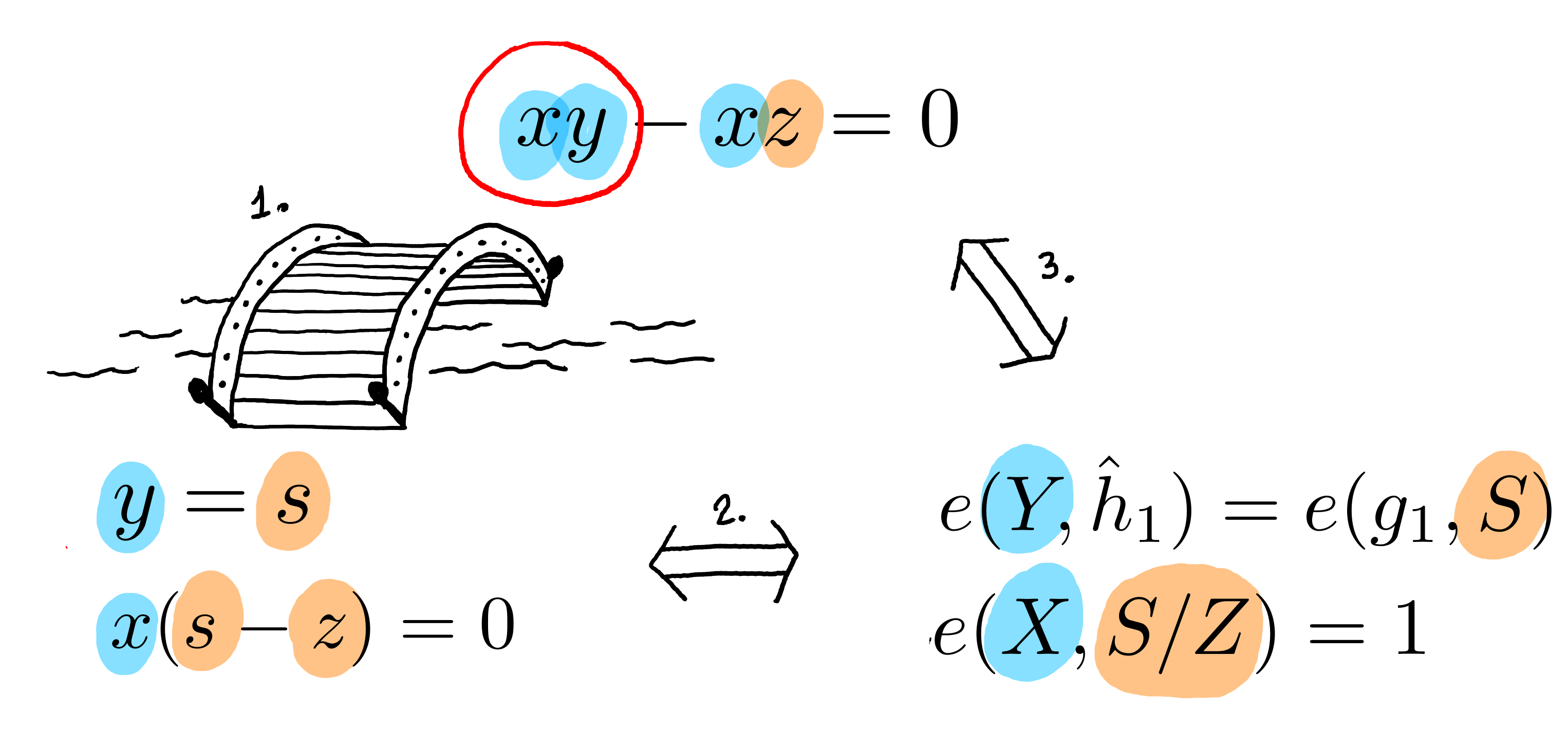
One characteristic feature of GS proofs is that all secret witness components must be group elements rather than field elements. So our secret that we want to keep hidden cannot be field elements $0$ or $1$ or $r$, but must instead be group elements $g_1^{0}$ or $g_1^1$ or $g_1^r$. For our ciphertext to encrypt $0$ or $1$ we thus desire that $m\in\{(g_1)^0,(g_1)^1\}$. Turning to the equation (1) we have that this condition that is equivalent to

where logarithm is taken with base $g_1$. Denote $W_2 = g_1^{w_2} = \mathsf{CT}_2\cdot \mathsf{pk}^{-\log \mathsf{CT}_1}$ We wish to check that $w_2^2-w_2 =0$. Our one and only method of checking constraints is using pairing equations. We cannot pair $W_2$ with itself because we can only pair $\mathbb{G}_1$ elements with $\mathbb{G}_2$ elements. Thus we choose to "bridge" $w_2$ into $\mathbb{G}_2$ by introducing an additional group element $\widehat{W}_3 = \widehat{h}_1^{\widehat{w}_3}$ such that

where $w_2$ is a logarithm of some $\mathbb{G}_1$ element $W_2$ and $\widehat{w}_3$ is a logarithm of some $\mathbb{G}_2$ element $\widehat{W}_3$.

Then (2) is equivalent to

That first condition in (3) that $\mathsf{CT}_2\cdot \mathsf{pk}^{-\log \mathsf{CT}_1} =W_2$ currently does not look very much like a pairing product equation. We cannot use logarithms in PPEs, so we need an alternative method for arithmetising that $\log \mathsf{CT}_2- \log \mathsf{CT}_1\cdot\log \mathsf{pk}=w_2$ As $\mathsf{CT}_1,\mathsf{CT}_2,\mathsf{pk}$ are all in $\mathbb{G}_1$, we make another bridge:

In pairing equations this is equivalent to

Combining all our pairing equations together we arrive at our final pairing product equation for arithmetising that $(\mathsf{CT}_1, \mathsf{CT}_2)$ encrypts $0$ or $1$.

General Proof Structure

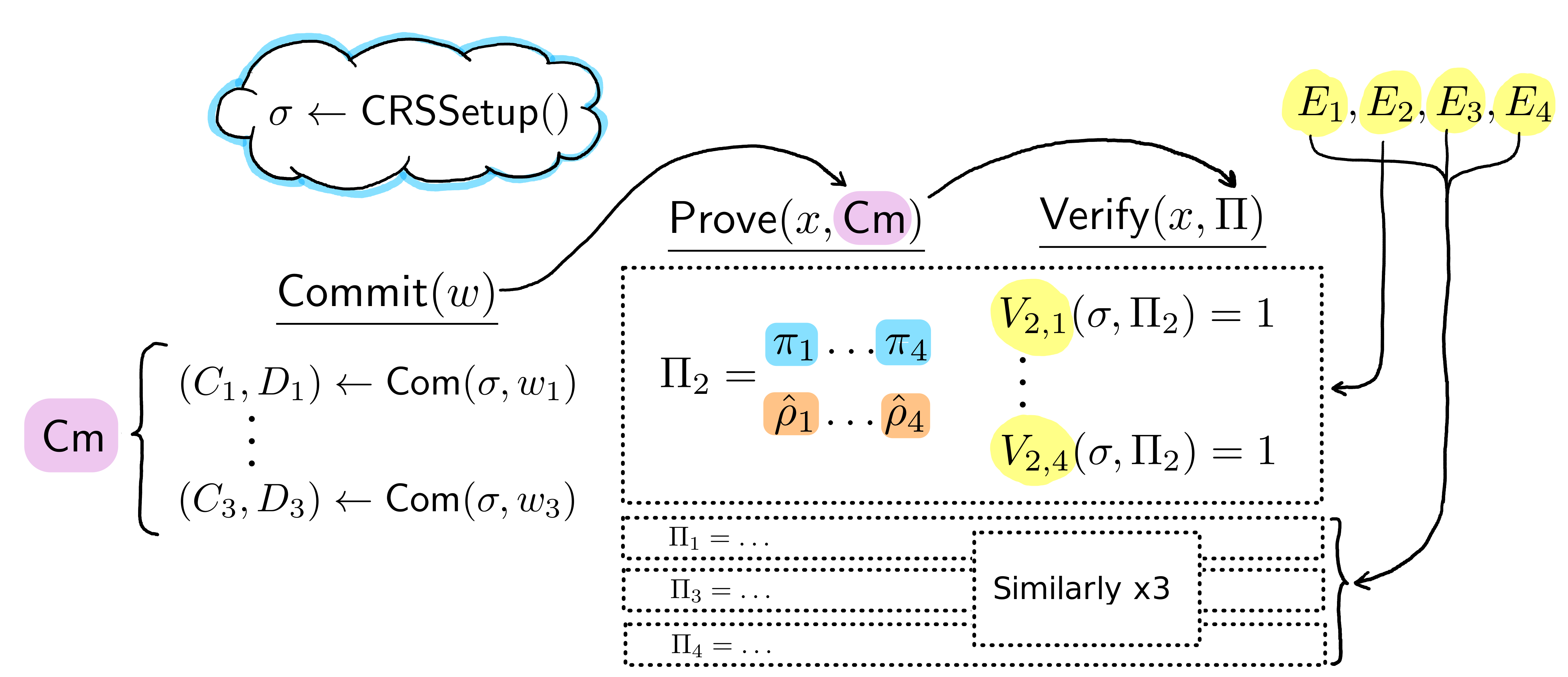
In this section we describe the GS setup, prover and the verifier used in representing the statement "This ciphertext encrypts $0$ or $1$".

Transparent Setup

We discuss how to run the GS setup. The setup does not depend on our pairing product equations at all and the same setup is used for proving any statement. It is only the prover and the verifier that depend on the pairing product equation explicitly.

NIZK proofs are constructed with a common reference string (CRS), that is used for both producing and verifying proofs. In GS proofs the CRS is constructed using public randomness and therefore they are said to have a trustless setup (this is a positive thing because we do not have to trust a third party or MPC that replaces it, like with many SNARKs). The GS CRS consists of eight independent elements --- four in each group.

In practice these elements are typically sampled as the output of a hash function, and the seed is published so that anyone can verify the setup procedure. It is permitted and encouraged to have fun (not too much fun) when choosing the seed and we sometimes like to use the opening lines of famous books.

We will reuse the generator $g_1$ for our ElGamal ciphertext which helps us to simplify the structure of prover and verifier.

Commitments to Witnesses

We now describe our GS prover. The prover aims to show the existence of a witness that satisfies the pairing product equations. The witness is secret and cannot be revealed directly. Thus instead the prover commits to the witness, and proves that the committed witness satisfies a related set of pairing product equations. We discuss the form of this commitment before we present the related set of equations.

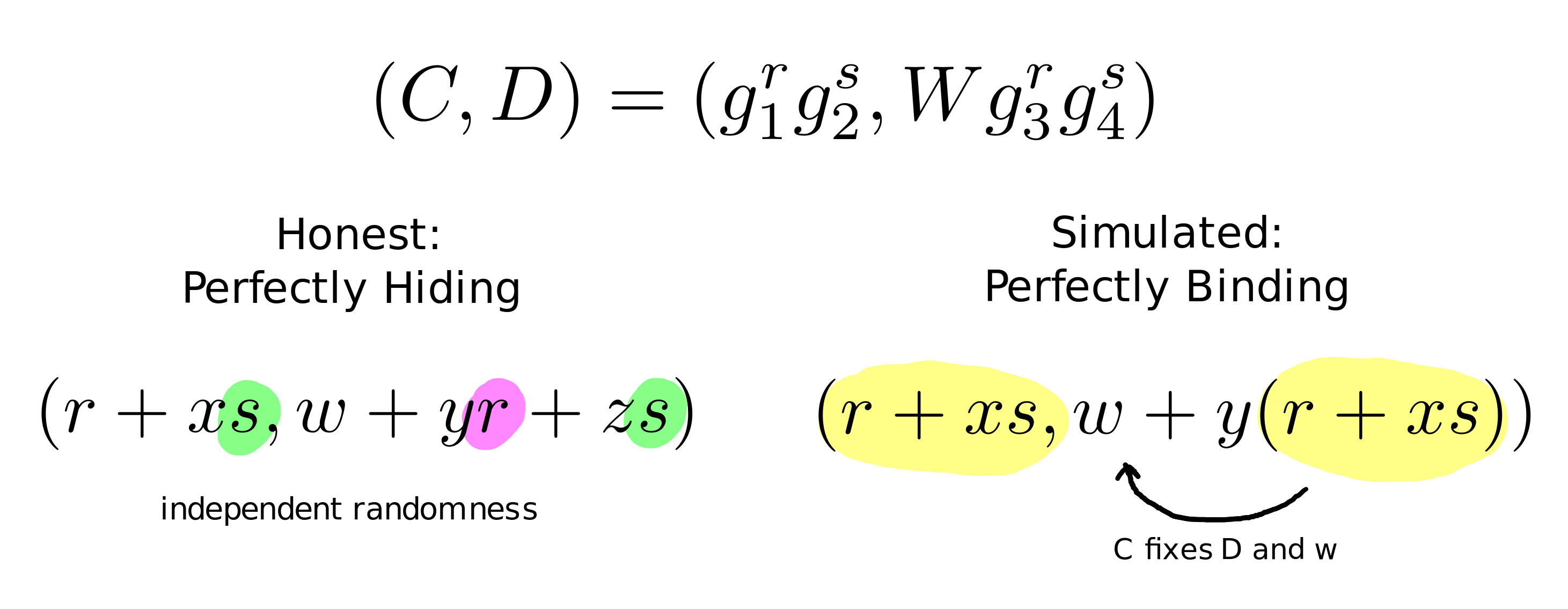
The prover computes two elements using an algorithm that looks a lot like ElGamal encryption. To commit to $W \in \mathbb{G}_1$ it chooses random field elements $r,s$, sets $C = g_1^r g_2^s, \ D = W g_3^r g_4^s$ and returns $(C,D)$. We have expressed the commitment with respect to $\mathbb{G}_1$. To commit to elements in $\mathbb{G}_2$ we use the same method with respect to the generators $(\widehat{h}_1\ldots \widehat{h}_4)$ instead of $(g_1\ldots g_4)$.

Typically when we present this commitment scheme to cryptographers their immediate response is "why two generators?" or "why not use Pedersen commitments?". The answer to this question is highly nuanced and answering it here would disrupt the flow of this explanation. Thus we're not going to. But as a teaser, we will say that Groth and Sahai describe this commitment scheme as one that either satisfies hiding or binding depending on how the setup parameters are chosen.

Now, in our particular case of ElGamal encryption, we commit to our witness $(\widehat{W_1}, W_2, \widehat{W_3})$ once for all equations $E_1-E_4$:

The Prover and The Verifier

While the commitments $(\widehat{C}_1, \widehat{D}_1, C_2, D_2, \widehat{C}_3, \widehat{D}_3)$ are shared across all pairing product equations, each pairing equation requires a unique set of $8$ proof elements and $4$ verifier equations, so forms a "sub-proof". Here, mostly to stay concise, we show and later derive the proof system (prover and verifier) only for the second equation $E_2$. For the full system thus, prover must produce proofs for all four equations, and verifier must verify them all.

Recall that $E_2$ has the form

The honest prover needs to construct the following eight elements, where $\alpha,\beta,\gamma,\delta$ are sampled randomly:

And the four equations $V_1 \ldots V_4$ the verifier must check on the commitments and proof elements are as follows:

The reader is encouraged to attempt deriving the same equations for $E_1,E_3$ which are both easier than our case (we put our derivation for them at the end of the blog post). A more sadistical writer might also ask the reader to derive equations for $E_4$ as an exercise (possibly hinting that it is a simple), but after having attempted this exercise for ourselves we realised that $E_4$ is more involved due to its quadratic component. Thus at the end of this document we will actively discuss $E_4$.

The form of proof elements and equations is somewhat homogeneous: we always have 8 proof elements and 4 verification equation per pairing equation, and the LHS of verification equations is always the same. However, the number of pairings in verification equations depends on the particular form of the pairing equation (reflected in the RHS). The commitments, as mentioned before, are generated once for all pairing equations, which amounts to 2 elements per witness element.

The following illustration shows how it works on a large scale:

Deriving Equations for $E_2$

The intention of this section is to provide an intuitive step-by-step explanation of how the proof elements and verification equations for the pairing product equation $E_2$ are derived. We describe our general strategy, but after that things are going to get more technical. To readers that don't fancy wading through pages of algebra, we recommend you stop reading after the general strategy is explained. To other readers who are more dedicated to understanding the magic behind GS proofs, we recommend you get comfortable with continously switching between additive and multiplicative notation because we do this a lot (we promise not in the same equation).

The General Strategy

We have a pairing product equation that the prover claims to hold for hidden witness variables. The prover cannot give the witness in the clear, this would violate zero-knowledge, but it still must tell the verifier something about its witness. The prover therefore generates a commitment which binds them to their witness without revealing any additional information.

Our general strategy now is to find an alternative set of pairing product equations that hold if and only if the contents of the commitments satisfy the original pairing product equation. Our strategy will proceed in two parts.

• During our first part we search for intemediary proof elements that satisfy an intermediary set of pairing product equations if and only if the contents of the commitment satisfy the original pairing product equation. We treat soundness as if it holds unconditionally i.e. as if the only way for the prover to cancel out the randomness from the CRS is to multiply by zero. In the formal proof, we actually show that soundness does hold unconditionally provided the CRS is chosen carefully.
• During our second part, we show how to randomise the intemediary proofs and pairing product equations in a way that fully hides the witness. This results in our final equations. Here we focus mostly on satisfying zero-knowledge but we must not break soundness in the process. In other words we try to ensure that a malicious verifier learns nothing from an honest prover, beyond the correctness of the ciphertext.

For arguing indistinguishability, one of the key properties we require is that the number of randomisers is equal to the number of proof elements minus the number of verifier equations. That way we can say e.g. that Element 1 is random, Element 2 is random, and Element 3 is the unique value satisfying Equation 1 given Elements 1 and 2. Thus our strategy is to add in additional randomisers to our proof elements and edit our verifier equations such that they still hold for the randomised proofs. To keep things sound we also have to add additional verifier equations to enforce that the prover doesn't abuse their newfound freedom. The other property we require is that there are no linear combinations between our randomisers such that they cancel out in undesirable ways. While deriving our equations for ($E_2$) we are merely going to optimistically hope that this holds, but formally check that it is the case later.

The Intemediary Pairing Product Equations for Commitments

For the first part of our strategy, we must find an intermediary set of pairing product equations demonstrating that the contents $(\widehat{W}_1, W_2)$ of the commitments

satisfy the second equation

For this explanation we find it helpful to work in logarithms, so here is some notation denoting the logarithms of generators in the CRS

Then the logarithms of our commitments are given by

If we now actually look at the logarithmic equation defined by ($E_2$) we get that

where $\mathsf{sk} = \log_{g_1}(\mathsf{pk})$. Notice that $r_1,s_1, s_2, r_2$ are known to the prover while $x,y,z,\widehat{u}, \widehat{v},\widehat{\ell}$ are not. We make no assumptions on whether $\mathsf{sk}$ is known to the prover or not.

Our derivation strategy is, by introducing new variables, to obtain a set of equations equivalent to $L_2$ such that

• The equations do not contain $\widehat{w}_1,w_2$;
• The equations are bilinear, i.e. each term has at most one variable from each group.

Step 1: We first express $\widehat{w}_1$ and $w_2$ in terms of the commitments $(\widehat{c}_1, \widehat{d}_1, c_2, d_2)$ and the randomness $\widehat{r}_1$, $\widehat{s}_1, r_2, s_2$. The commitment $\widehat{D}_1$ should use the same randomness $\widehat{r}_1$, $\widehat{s}_1$ as the commitment $\widehat{C}_1$. Therefore, we substitute $r_1 = \widehat{c}_1 - \widehat{u} s_1$ into the equation for $\widehat{w}_1$ and obtain:

Similarly for the second commitment: $w_2 = d_2 - (c_2 - x s_2) y - s_2 z$

Step 2: Substituting into $(L_2)$ we get

Step 3: The terms $\log{\widehat{\mathsf{CT}}_2}, \mathsf{sk} \cdot \widehat{d}_1, d_2$ are already in the pairing equation form (degree at most two, at most two elements from different groups), so we leave them alone, moving to the RHS, and swapping sides of the equation:

Now, we want the RHS summands to be in the pairing-friendly form too. Currently they are not. For example, we cannot pair $C_2$ with $g_3 = g_1^y$ because these are both in the same source group.

Step 4: To get the RHS into a pairing friendly form, we will introduce new elements. For each summand we introduce one proof element. For example, where $y$ is multiplied by $(c_2 - x s_2)$, we introduce $\widehat{\phi}_1' = c_2 - s_2 x$. This suggests creating four additional elements:

The additional proof elements we introduced is somewhat arbitrary --- there are many (closely related if not equivalent) ways to construct GS verification equations. Now our first equation is in the following well-formed pairing-compatible form:

Step 5: Our fifth and final step for determining the intemediary pairing equations is to enforce the previous four equations for $\Theta_1',\Theta_2',\widehat{\Phi}_1',\widehat{\Phi}_2'$. We start by joining the first two (substituting the second into the first) and obtaining: $\theta_1' = \mathsf{sk} \cdot \widehat{c}_1 - \theta_2' \widehat{u}$ Similarly, by joining the third and the fourth equations, we get:

Resulting Intemediary Pairing Product Equation: Putting all $5$ steps together, our intemediary pairing product equation challenges the prover to find

such that they satisfy

(Proof elements in verification equations are without primes since they are considered to be formal variables.) Together these show that the commitments $(\widehat{C}_1, \widehat{D}_1)$ and $(C_2, D_2)$ contain witness elements $\widehat{W}_1$ and $W_2$ such that the second pairing product equation ($E_2$) is satisfied.

We are now going to frustrate the reader by observing that the above process was rather circular. Indeed we cannot reveal $\Theta_1', \Theta_2', \widehat{\Phi}_1', \widehat{\Phi}_2'$ in the clear: they reveal too much information about the witness and violate zero-knowledge. For example observe that

for $m$ our secret message. The next step, however, will not be circular and we will show how to randomise these proof components in a manner that does not break zero-knowledge. That we have really gained is that $\Theta_1', \Theta_2', \widehat{\Phi}_1', \widehat{\Phi}_2'$ depend only on the original pairing product equations and the commitment randomness $r_1, s_1, r_2, s_2$. In particular they do not depend on the witness $\widehat{W}_1$, $W_2$.

A general property that is required (but not sufficient!) for zero knowledge is that number of randomisers $\geq$ number of proof elements $-$ number of verification equations. Here we have $4$ commitment elements with $4$ randomisers and then $4$ proof elements with no additional randomisers. Given $3$ verifier equations this leaves us $1$ randomiser short.

Adding Zero-Knowledge: Getting Sufficient Randomisers

For the second part of our strategy, we must randomise our intermediary proofs $(\Theta_1', \Theta_2', \widehat{\Phi}_1', \widehat{\Phi}_2')$ and pairing product equations $(V_1'), (V_2'), (V_3')$ to keep the witness hidden. We do this by adding blinding factors to $\Theta_1',\Theta_2'$ (order does not matter), and cancelling out the additional noise using other proof elements. Often the only way we can balance the randomised pairing equations is by adding additional proof elements. When we do this, we either add at least one new randomiser to the new proof element, or a new verifier equation which is a quadratic combinations of our other proof elements.

Step 1: We first introduce a randomiser to $\Theta_1'$. We must then edit our intemediary equations to adjust for the extra randomness. We set

By substituting this into the RHS of $(V_1')$

we see that an additional term $y \alpha \widehat{v}$ has been acquired. This is unwanted noise that we must cancel out. To cancel the extra terms we edit $\widehat{\phi}_1'$ accordingly

because this term is multiplied by $y$. Now $(\Theta_1'', \Theta_2', \Phi_1'', \Phi_2')$ satisfy $(V_1')$ and do not reveal the witness.

Step 2: We edit $(V_2')$ so that our randomised proof elements can satisfy it. The RHS of $(V_2')$ is given by

and this has aquired the additional noise $y \alpha$. We cannot hope to cancel this noise out with $\Theta_2$ because of the $\widehat{u}$ multiplier. For soundness, we also want to enforce that the noise added in $\Theta_1''$ is actually a multiple of $y$ and does not interfere with the witness. We thus introduce a new proof element that will be paired with $y$ blinded by an additional randomiser $\gamma$

And therefore, $(V_2'')$ becomes

Now $\widehat{\phi}_3$ does not prevent $(V_2')$ from being satisfied whenever $(V_2'')$ is satisfied because $y$ is an unused basis. To make this equation balance we modify $\Theta_2'$ and get

and we see $(V_2'')$ is still satisfied.

Step 3: We look back at $(V_1')$ with respect to our randomised proof element $\Theta_2''$. By substituting this into the RHS of $(V_1')$

we see that an additional term $\gamma y \widehat{\ell}$ has been acquired. This is unwanted noise that we must cancel out. To cancel the extra terms we edit $\widehat{\phi}_1''$ accordingly

because this term is multiplied by $y$. Now $(\Theta_{1}'', \Theta_2', \Phi_1, \Phi_2')$ satisfy $(V_1')$ and do not reveal the witness.

Step 4: We edit $(V_3')$ so that our randomised proof elements can satisfy it. The RHS of $(V_3')$ is given by

and this has aquired the additional noise $-\alpha \widehat{v} - \gamma \widehat{l}$. To cancel out the extra noise we introduce two new proof elements that will be paired with $\widehat{v}$ and $\widehat{l}$ respectively, and blind them with $\beta$ and $\delta$

And therefore, $(V_3')$ becomes

Now $\Theta_3, \Theta_4$ does not prevent $(V_3')$ from being satisfied whenever $(V_3)$ is satisfied because $\widehat{v}, \widehat{\ell}$ is an unused basis. To make this equation balance we modify $\widehat{\phi}_2$:

and we see $(V_3)$ is still satisfied.

Step 5: We look back at $(V_1')$ with respect to our randomised proof element $\widehat{\phi}_2$. By substituting this into the RHS of $(V_1')$

we see that an additional term $- \beta z \widehat{v} - \delta z \widehat{\ell}$ has been acquired. This is unwanted noise that we must cancel out. To cancel the extra terms we edit $\Theta_1''$ and $\Theta_2''$ accordingly

Now $(\Theta_{1}, \Theta_2, \Phi_1, \Phi_2)$ satisfy $(V_1')$ and do not reveal the witness.

Step 6: We edit $(V_2'')$ so that our randomised proof elements can satisfy it. The RHS of $(V_2'')$ is given by $\theta_1 + \theta_2 \widehat{u} + y \widehat{\phi}_3$ and this has aquired the additional noise $\beta z + \delta z \widehat{u}$.

We shall need to add a proof element which is paired with $z$ to cancel the noise. We cannot balance any additional randomness that this new element introduces because $\Theta_1$ and $\Theta_2$ already both have $z$ components. Thus for our final proof element to not use up a randomiser we instead add a verification equation. See that

We thus introduce a new proof element

and a verification equation

Now $(V_2'')$ becomes

We do not need to edit $(V_1')$ or $(V_3)$ because no proof elements have been edited.

Resulting Verifier Equations: Putting everything together, we have the following eight proof elements

and $4$ verification equations

The verification equations $(V_1), (V_2), (V_3), (V_4)$ given in Section 3 are exactly equal to what we have just derived.

This completes our explanation for how the prover and verifier for $(E_2)$ are derived. In the next sections we will dive into the security rationale behind this construction, and give more formal arguments of security than simply stating that we have the correct number of randomisers. Still, if you are constructing a zero-knowledge proof but have less randomisers than proof elements minus verifier equations, then it is time to become very suspicious of your result.

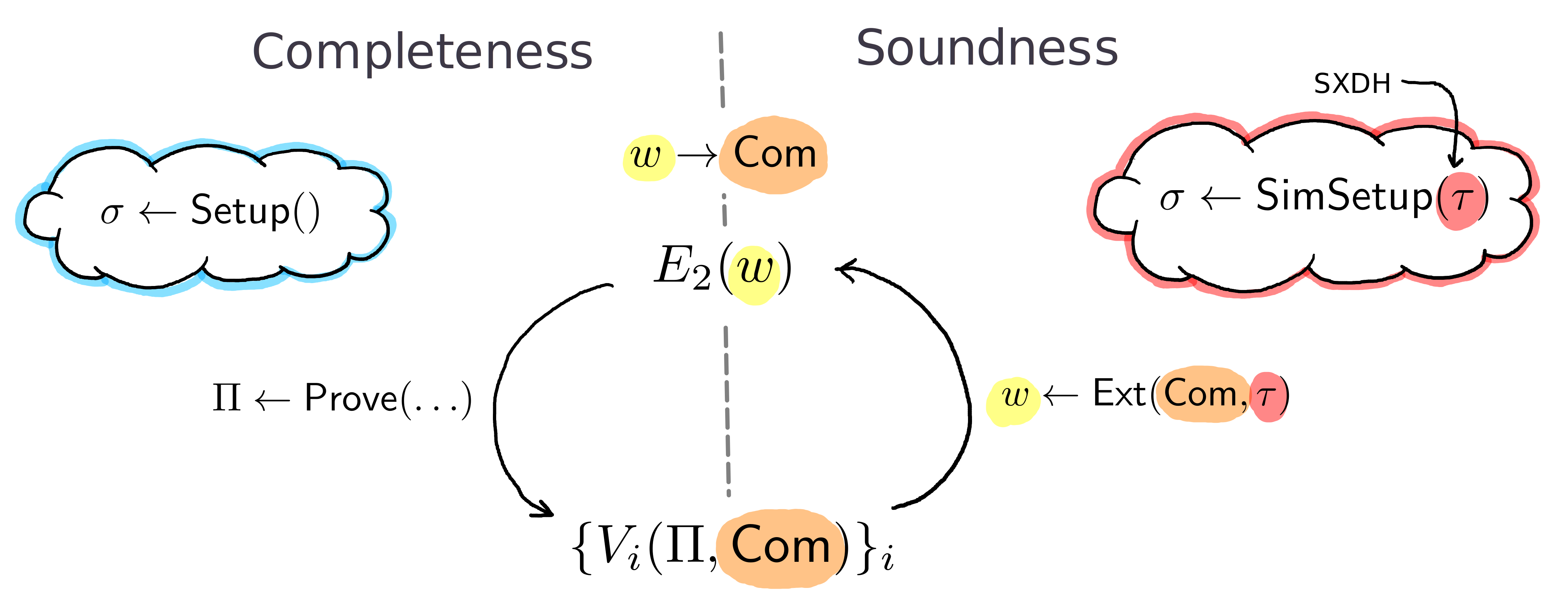
Proving Security

The previous section explains how, intuitively, one should arrive at GS equations, using $E_2$ as an example input equation. Now we explain (and formally prove) why the resulting system of equations satisfies completeness, soundness, and zero-knowledge.

Completeness

(Does anyone ever actually prove completeness? The proofs satisfy the verifier in our implementation...)

Completeness of the proof system means that every honestly-generated proof verifies with probability one. That is, if $W_1,W_2,W_3$ satisfy $E_2$, then $\vec\Pi = (\vec\Theta,\vec\Phi)$ satisfies $V_1 \land V_2 \land V_3 \land V_4$. It can be easily seen that this holds by construction because proof elements that satisfy the original equations (commitment validity + $(E_2)$) must also satisfy the derived equations.

Soundness

Soundness of the non-interactive proof system means that for any adversarially constructed proof that verifies there exists a witness to the given relation (in our case, the witness is ($\widehat{W}_1, W_2$)). The GS proof that we presented, like with most of the common zero-knowledge proofs today, is computationally sound assuming that a cryptographic problem is hard. The assumption here is the SXDH (Symmetric External Diffie-Hellman): nobody can tell the difference between random $(g_1,g_2,g_3,g_4)$ and $(g_1,g_1^x,g_1^y,g_1^{xy})$ in $\mathbb{G}_1$ and analogously for $\mathbb{G}_2$. Looking ahead, this will help us argue that a commitment setup $\left ( (g_1,g_1^x,g_1^y,g_1^{xy}),(\widehat{h}_1,\widehat{h}_1^{\widehat{u}},\widehat{h}_1^{\widehat{v}},\widehat{h}_1^{\widehat{u} \widehat{v} }) \right )$ looks similar to $\left ( (g_1,g_2,g_3,g_4),(\widehat{h}_1,\widehat{h}_2,\widehat{h}_3,\widehat{h}_4) \right )$.

The intuition about soundness can be found in the way the equations $V_1 \ldots V_4$ were constructed. We built them such that when the original $E_2$ holds for some witness elements, the final $\{V_i\}_i$ hold too ($E_2 \Rightarrow \{V_1 \ldots V_4\}$). But the transformations that we applied to our equations are in fact one-to-one, and it is also true that when $\{V_i\}_i$ hold, $E_2$ holds for some witness ($\{V_1 \ldots V_4\} \Rightarrow E_2$).

To formally demonstrate soundness, the only cryptographically elaborate detail is to show that $(\widehat{C}_1,\widehat{D}_1), (C_2, D_2)$ are always commitments that contain some $\widehat{W}_1, W_2$ and not some stray elements. This is where SXDH comes in play. The reader can follow a more formal assertion of soundness in the hidden section next.

Collapsible: Commitment scheme under standard and SXDH setups.

The commitment scheme with the standard setup, where all base elements are randomly picked, is perfectly hiding and computationally binding. Because of this, when we see a commitment under standard setup, intuitively, we cannot claim that anything is "contained" inside of it, which is necessary for the existentially qualified soundness statement: "for every verifying proof there exists a witness". We only know that for whatever was put in there, it's computationally impossible for the prover to find another element that this commitment opens to. Put more explicitely, upon seeing a commitment $(\widehat{C}_1, \widehat{D}_1)$ we cannot extract some unique $\widehat{W}_1$ such that the commitment contains $(\widehat{h}_1^{r_1} \widehat{h}_2^{s_1}, \widehat{W}_1 \widehat{h}_3^{r_1} \widehat{h}_4^{s_1})$ because there are multiple solutions.

When instantiated with the SXDH setup though $(g_1,g_1^x,g_1^y,g_1^{xy}),(\widehat{h}_1,\widehat{h}_1^{\widehat{u}},\widehat{h}_1^{\widehat{v}},\widehat{h}_1^{\widehat{u} \widehat{v}})$, the commitment scheme becomes, in contrast, computationally hiding and perfectly binding. Comparing to the previous situation, we know that for every commitment, there is exactly one valid element committed that can lead to this outcome (one-to-one correspondence). This is just as an encryption scheme (actually it is literally ElGamal encryption). This means that we, knowing the alternative setup trapdoors $(x,y, \widehat{u}, \widehat{v})$, can decrypt the commitments and obtain the witness.

Our strategy for proving soundness is therefore to show that we can extract a witness that satisfies $E_2$ from any proof that is valid for the SXDH (=subverted) setup. One extracts a witness by decrypting the commitments (see step 1 below), and shows it is a witness by checking $V_1$-$V_4$ equations (step 2 below). The strategy proves the soundness for not only SXDH setups but for any setups that are indistinguishable from such. The SXDH assumption tells us that any random setup should be as such, and thus we prove the soundness. Now back to the witness:

• First of all, each pair of elements $(C_2,D_2) \in \mathbb{G}_1 \times \mathbb{G}_1$ is a proper perfectly binding commitment. It is easy to see that with $c_2 = r_2 + x s_2$ we have $d_2 = w_2 + y r_2 + x y s_2 = w_2 + y c_2$. This means that in honestly constructed commitments under SXDH the second element is always deterministically defined by the first. As argued for any $(C_2,D_2)$ there always exist $w_2$ such that $(C_2,D_2) = \mathsf{Commit}(g_1^{w_2},(r_2,s_2)) = (g_1^{r_2 + x s_1}, g_1^{w_2} g_1^{y (r_2 + x s_2 ) })$ for some $r_2,s_2$. Similarly, $(\widehat{C}_1,\widehat{D}_1) = \mathsf{Commit}(h_1^{\widehat{w}_1},(r_1,s_1)) = (\widehat{h}_1^{r_1 + \widehat{u} s_1}, \widehat{h}_1^{\widehat{w}_1} \widehat{h}_1^{\widehat{v} (r_1 + \widehat{u} s_1 )})$.

• Now we review $V_1 \ldots V_4$ in logarithms with commitment representations given:

$$\begin{array}{cl} \theta_1\widehat{v} + \theta_2\widehat{u}\widehat{v} + y\widehat{\phi}_1 + xy \widehat{\phi}_2 &= \underbrace{w_2 + y c_2}_{d_2} - \log{\mathsf{CT}_2} + \mathsf{sk} \underbrace{(\widehat{w}_1 + \widehat{v} \widehat{c}_1)}_{\widehat{d}_1}\\ \theta_1 + \theta_2\widehat{u} + y\widehat{\phi}_3 + xy \widehat{\phi}_4 &= \mathsf{sk} \cdot \widehat{c}_1\\ \theta_3\widehat{v} + \theta_4\widehat{u}\widehat{v} + \widehat{\phi}_1 + x \widehat{\phi}_2 &= c_2\\ \theta_3 + \widehat{u} \theta_4 + \widehat{\phi}_3+ x\widehat{\phi}_4 &= 0 \end{array}$$

Performing arithmetic operations on both sides of each equation simultaneously, $V_1 - V_2 \cdot \widehat{v} - V_3 \cdot y$ is equal to:

$$-\widehat{v}(y \widehat{\phi}_3 + xy \widehat{\phi}_4) - y(\theta_3 \widehat{v} + \theta_4 \widehat{u} \widehat{v}) = w_2 + \mathsf{sk} \cdot \widehat{w}_1 - \log{\mathsf{CT}_2}$$

LHS of which is exactly $\widehat{v} y V_4$, and since $V_4 = 0$, the left hand side is 0. So in the end we obtain, on the RHS, $w_2 + \mathsf{sk} \cdot \widehat{w}_1 - \log{\mathsf{CT}_2} = 0$ as expected from $E_2$.